
| 일 | 월 | 화 | 수 | 목 | 금 | 토 |
|---|---|---|---|---|---|---|
| 1 | 2 | 3 | ||||
| 4 | 5 | 6 | 7 | 8 | 9 | 10 |
| 11 | 12 | 13 | 14 | 15 | 16 | 17 |
| 18 | 19 | 20 | 21 | 22 | 23 | 24 |
| 25 | 26 | 27 | 28 | 29 | 30 | 31 |
Tags
- Loss Function
- react native
- Expo
- marksense.ai
- @Transactional
- 2021 제9회 문화공공데이터 활용경진대회
- skt fellowship 3기
- google cloud
- AWS
- html
- Spring Boot
- matplotlib
- JPA
- idToken
- YOLOv5
- 커스텀 데이터 학습
- 코드업
- pandas
- yolo
- javascript
- OG tag
- 졸프
- Spring
- oauth
- C++
- google login
- 순환참조
- STT
- google 로그인
- 양방향 매핑
Archives
- Today
- Total
민팽로그
성능 향상을 위한 데이터 스케일링 본문
데이터셋은 아래 링크에서 구할 수 있음
https://archive.ics.uci.edu/ml/index.php
UCI Machine Learning Repository
Welcome to the UC Irvine Machine Learning Repository! We currently maintain 588 data sets as a service to the machine learning community. You may view all data sets through our searchable interface. For a general overview of the Repository, please visit ou
archive.ics.uci.edu
- linear_regression: 직선으로 표현 가능한 수식. y = wx + b. x 컬럼 1개와 y 컬럼 1개일 때 사용하기 좋음.
- multiple_regression: 2개 이상의 x컬럼과 1개의 y컬럼 및 예측값이 2개 이상일 때 사용하기 좋음.
- logistic_regression: 2개 이상의 x컬럼과 1개의 y컬럼 및 이진분류(0, 1)일 때 사용하기 좋음. 손실 함수로 binary_crossentropy 사용.
- softmax_regression: 2개 이상의 x컬럼과 3개 이상의 y컬럼 및 예측값이 2개 이상일 때 사용하기 좋음. 출력층 활성화 함수로 softmax, 손실 함수로 categorical_crossentropy 사용.
adult 데이터셋 - 50세 이상인지 예측
import tensorflow.keras as keras
import numpy as np
import pandas as pd
from sklearn import preprocessing


def get_data_encoder(file_path):
    # 파일 읽기
    names = ['age', 'workclass', 'fnlwgt', 'education', 'education-num',
             'marital-status', 'occupation', 'relationship', 'race',
             'sex', 'capital-gain', 'capital-loss', 'hours-per-week',
             'native-country', 'income']
    adult = pd.read_csv(file_path,
                        names=names,
                        sep=', ',
                        engine='python')  # sep가 2글자 이상이기 때문에 기본적으로 사용하는 c 엔진에서 파이썬 엔진으로 바꿔줘야 함
    # print(adult)

    # print(adult.values[:5, 0])        # [39 50 38 53 28]
    # print(adult.values[:5, 1])        # ['State-gov' 'Self-emp-not-inc' 'Private' 'Private' 'Private']

    # print(adult['age'].values)

    # adult.info()

    # 6행 32561열 : 전치(transpose)되어있음
    x = [adult['age'].values, adult['fnlwgt'].values,
         adult['education-num'].values, adult['capital-gain'].values,
         adult['capital-loss'].values, adult['hours-per-week'].values]
    x = np.int32(x)
    # print(x[:, :5])

    x = np.transpose(x)
    # print(x.shape, x.dtype)     # (32561, 6) int32
    # print(x[:5, :])

    enc = preprocessing.LabelEncoder()
    y = enc.fit_transform(adult['income'].values)
    # print(y[:10])

    # 문자열 데이터를 x 데이터에 추가
    workclass = enc.fit_transform(adult['workclass'].values)
    education = enc.fit_transform(adult['education'].values)
    marital = enc.fit_transform(adult['marital-status'].values)
    occupation = enc.fit_transform(adult['occupation'].values)
    relationship = enc.fit_transform(adult['relationship'].values)
    race = enc.fit_transform(adult['race'].values)
    sex = enc.fit_transform(adult['sex'].values)
    native = enc.fit_transform(adult['native-country'].values)

    added = [workclass, education, marital, occupation, relationship, race, sex, native]
    # added = np.array(added)
    # print(added.shape)
    added = np.transpose(added)
    print(added.shape, added.dtype)     # (16281, 8) int32

    x = np.concatenate([x, added], axis=1)

    x = preprocessing.minmax_scale(x)  # 단위가 다르면 스케일링 꼭 고려! minmax_scale, scale 중 잘나오는거 사용

    return x, y


# 똑같은 데이터를 원핫 벡터로 바꾸면 일반적으로 성능이 조금 더 좋아짐
def get_data_binarizer(file_path):
    names = ['age', 'workclass', 'fnlwgt', 'education', 'education-num',
             'marital-status', 'occupation', 'relationship', 'race',
             'sex', 'capital-gain', 'capital-loss', 'hours-per-week',
             'native-country', 'income']
    adult = pd.read_csv(file_path,
                        names=names,
                        sep=', ',
                        engine='python')
    # print(adult)

    # print(adult.values[:5, 0])        # [39 50 38 53 28]
    # print(adult.values[:5, 1])        # ['State-gov' 'Self-emp-not-inc' 'Private' 'Private' 'Private']

    # print(adult['age'].values)

    # adult.info()

    x = [adult['age'].values, adult['fnlwgt'].values,
         adult['education-num'].values, adult['capital-gain'].values,
         adult['capital-loss'].values, adult['hours-per-week'].values]
    x = np.int32(x)
    # print(x[:, :5])

    x = np.transpose(x)
    # print(x.shape, x.dtype)     # (32561, 6) int32
    # print(x[:5, :])

    enc = preprocessing.LabelBinarizer()
    y = enc.fit_transform(adult['income'].values)
    # print(y[:10])

    bi = preprocessing.LabelBinarizer()
    workclass = bi.fit_transform(adult['workclass'].values)
    education = bi.fit_transform(adult['education'].values)
    marital = bi.fit_transform(adult['marital-status'].values)
    occupation = bi.fit_transform(adult['occupation'].values)
    relationship = bi.fit_transform(adult['relationship'].values)
    race = bi.fit_transform(adult['race'].values)
    sex = bi.fit_transform(adult['sex'].values)
    # train과 test 클래스 갯수가 달라서  skip
    # print(native.shape, sex.shape)      # (32561, 42) (32561, 1)

    x = np.concatenate([x, workclass, education, marital, occupation, relationship, race, sex], axis=1)
    x = preprocessing.minmax_scale(x)  # 단위가 다르면 스케일링 꼭 고려! minmax_scale, scale 중 잘나오는거 사용

    return x, y


# x_train, y_train = get_data_encoder('data/adult.data')
# x_test, y_test = get_data_encoder('data/adult.test')
# print(x_train.shape, y_train.shape)   # (32561, 14) (32561,)
# print(x_test.shape, y_test.shape)     # (16281, 14) (16281,)

x_train, y_train = get_data_binarizer('data/adult.data')
x_test, y_test = get_data_binarizer('data/adult.test')
# print(x_train.shape, y_train.shape)     # (32561, 65) (32561, 1)
# print(x_test.shape, y_test.shape)       # (16281, 65) (16281, 1)

# 읽어온 데이터에 대해 모델을 구축
model = keras.Sequential()
model.add(keras.layers.Dense(32, activation='relu'))
model.add(keras.layers.Dense(12, activation='relu'))
model.add(keras.layers.Dense(1, activation='sigmoid'))

model.compile(optimizer=keras.optimizers.Adam(0.001),
              loss=keras.losses.binary_crossentropy,
              metrics='acc')

model.fit(x_train, y_train, epochs=100, verbose=2,
          batch_size=100,
          validation_data=(x_test, y_test))
print(model.evaluate(x_test, y_test, verbose=0))
스케일링한 부분

데이터 스케일링 전

데이터 스케일링 후
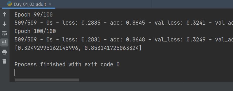
-> 정확도가 1.8%정도 증가함
'머신러닝&딥러닝' 카테고리의 다른 글
| 10월 6일 언어 지능 실습 (0) | 2021.10.06 |
|---|---|
| 10월 1일 언어 지능 실습 (0) | 2021.10.02 |
| optimizer (0) | 2021.10.01 |
| 9월 30일 언어 지능 실습 (0) | 2021.10.01 |
| 9월 29일 언어 지능 실습 (0) | 2021.09.29 |
'머신러닝&딥러닝' Related Articles
more

Comments